A posteriori estimator distinguishing different error components and adaptive stopping criteria
The Laplace problem: distinguishing the algebraic and discretization error components
This is the simplest case of the theoretical work of Ern and Martin (2013): ADAPTIVE INEXACT NEWTON METHODS WITH A POSTERIORI STOPPING CRITERIA FOR NONLINEAR DIFFUSION PDES . You can find here a modified version based on the implementation work of Martin Čermák.
Here, we will show you how to do implementer the error estimator and the stopping criteria with the software Freefem++ for the Laplace problem. The estimator can distinguish the different error components in the computation, respectively the algebraic and discretization error parts.
Let $\Omega\subset \mathbb{R}^2$ be an open bounded polygonal domain with the boundary denoted by $\partial \Omega$. Let us consider here the Laplace equation: for $f\in L^2(\Omega)$, find $u: \Omega \rightarrow \mathbb{R}$ such that $$\begin{align} -\Delta u = f &\qquad \mbox{ in }\Omega, \\ u = 0 & \qquad \mbox{ on } \partial\Omega. \end{align} $$ The variational formulation is defined by: Find $u\in H^1_0(\Omega)$ such that $$ (\nabla u, \nabla v) = (f,v) \qquad \forall v\in H^1_0(\Omega). $$ We denote by $\mathcal{T}_h$ the mesh used in the following. $\mathcal{T}_h$ is a simplicial partition of the polytope $\Omega$, i.e. $\cup_{K\in\mathcal{T}_h} \overline{K} = \overline{\Omega}$, any $K\in\mathcal{T}_h$ is a closed simplex (a triangle in 2D), and the intersection of two different simplices is either empty (a vertex, an edge in 2D).
For this example, we consider the $\mathbb{P}_1$-conforming finite element method, that means we shall be using $V_h\subset H^1_0(\Omega)$ $$ V_h=\mathbb{P}_1(\mathcal{T}_h)\cap H^1_0(\Omega) = \left\{v_h\in H^1_0(\Omega); v_h\mid_K\in \mathbb{P}_1(K), \qquad K\in \mathcal{T}_h\right\}. $$
Using the finite element method, the discrete variational formulation is given by: Find $u_h\in V_h$ such that $$ (\nabla u_h, \nabla v_h) = (f,v_h) \qquad \forall v\in V_h. $$ Now we get a linear algebraic system to solve, as $A u_h=b$.
When we want to solve the algebraic system, as the size of the matrix $A$ is large in practice, so we use some iterative methods, as CG method, GMRES method etc. The precision of the algebraic solve depends on the number of iterations in the algebraic solver.
As shown in the classic case, with a given mesh, we have already the discretization error, and this error depends only on the quality of the mesh.
As the total numerical error is the sum of the discretization error and the algebraic error. So in practice, it is not necessary to have too much iterations in the algebraic solver, as the discretization error do not change. The idea of this work is to stop the iteration in the algebraic solver when the algebraic error do not have significant influence to the total error.
In the following, I will show some extraction of the full script to help understand the implementation work. Firstly, we define the mesh and the variational formulation:
// mesh
int numnode=40;
mesh Th = square(numnode,numnode);


fespace Uh(Th,P1);  // function space for  u
Uh u, uh;
Uh uhp, uDisc;   // udisc solution by exact solver;  uhp solution by adaptive inexact solver

fespace Wh(Th,P0);  // function space for show the distribution map


// Definition FOR MACRO
macro Div(u1,u2) (dx(u1)+dy(u2)) //EOM
macro Grad(u) [dx(u),dy(u)]      //EOM


// Data for the given problem
func uExact = x*(x-1)*y*(y-1);
func dxduExact=(2*x-1)*y*(y-1);
func dyduExact=(2*y-1)*x*(x-1);
func f = -2*(x*x+y*y)+2*(x+y);

varf a(u,v)=int2d(Th)(Grad(u)'*Grad(v)) + int2d(Th)(f*v) + on(1,2,3,4,u=uExact);
varf BC(u,v)=on(1,2,3,4,u=1);
matrix A=a(Uh,Uh,tgv=-1,solver=GMRES);
real[int] BC1=BC(0,Uh,tgv=-1);
We can solve it exactly, as follows
int nbCG;  // nb of iteration for ExactSolver
func int ExactSolver()
{
cout<<" ********* Exact LinearCG solver ********* " << endl;
    func real[int] DJ(real[int] &u)
    {
	real[int] Au=A*u;
	return Au;
    };


    func bool stop1(int iter, real[int] u, real[int] g) {
	nbCG=iter;
	return 0;
    }


    real[int] b=a(0,Uh,tgv=-1);
    u[] = BC1 ? b : 0;

    real tmptime=clock();
    LinearCG(DJ,u[],b,eps=1.e-8,nbiter=10000,verbosity=5,stop=stop1);
    cout<<"we need the computation time = "<< clock()-tmptime<< endl;
    uDisc[]=u[];

    plot(uDisc,value=1,fill=1,cmm="Discrete solution");
    cout<<" The number of iterations we need is = "<< nbCG<< endl;
    cout<<"\n\n"<< endl;

}
ExactSolver();
We can use also the adaptive inexact solver, as done in the following
// Parameter for Stopping criterion
real GammaRem=0.5, GammaAlg=0.5;
int nu=10;

func int AdaptiveSolver()
{
cout<<" ********* Adaptive LinearCG solver ********* " << endl;


    func bool stop(int iter, real[int] u, real[int] g){
        // we check the error estimation every nu step, and we begin from nu-th step
	if (iter%nu==0 && iter>0){
	    uh[]=u;
	    stopcriteria=estimation(iter);
	}
	if (stopcriteria>0){
	    return 1;
	}
	return 0;
    }


    func real[int] DJ(real[int] &u)
    {
	real[int] Au=A*u;
	return Au;
    };

    real[int] b=a(0,Uh,tgv=-1);
    u[] = BC1 ? b : 0;
    LinearCG(DJ,u[],b,eps=1.e-8,nbiter=10000,verbosity=5,stop=stop);

   }

AdaptiveSolver();
As you see in the script, using the function "stop" I define the stopping criterion for the algebraic solver, with the help of the function "estimation", which can be defined as follows:
    func int estimation(int innernum)
    {
	if (innernum==nu){
	    RHSd();
	    uhp = uh;                                 // set uhp=uh
	    real etaDisc  = ComputeEtaDisc(innernum); // compute etaDisc
	    etaDiscSave  = etaDisc;
	    [sigma1p,sigma2p]=[sigma1,sigma2];
	}
	else{
	    RHSd();
	    real etaRem=ComputeEtaRem(innernum);     // compute etaRem, we need uhp and uh
	    real etaAlg=ComputeEtaAlg(innernum);     // compute etaAlg, we need uhp and uh

	    real maxError=max(etaAlg,etaDiscSave);
	    if(etaRem>GammaRem*maxError){            // search uh which satisfy the stopping criterion: finish the computation or change uhp=uh
		return 0;
	    }else{
		if (etaAlg>GammaAlg*etaDiscSave){
		    uhp = uh;
		    nbCGinexact=innernum;  // the lastest step where we stop the computation
		    real etaDisc= ComputeEtaDisc(innernum);
		    etaDiscSave=etaDisc;
		    [sigma1p,sigma2p]=[sigma1,sigma2];
		    return 0;
		}else{
		    real etaDisc= ComputeEtaDisc(innernum);
		    return 1;
		}
	    }
	}
	return 0;
    }
And the results
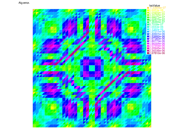
  -- Square mesh : nb vertices  =1681 ,  nb triangles = 3200 ,  nb boundary edges 160
 ********* Exact LinearCG solver *********
CG converges 64  ro = 0.380329 ||g||^2 = 2.73212e-20 stop=0 /Stop= 0x1a6e5d0
 The number of iterations we need is = 64


 ********* Adaptive LinearCG solver *********
CG converges 40  ro = 0.376054 ||g||^2 = 2.34935e-11 stop=1 /Stop= 0x43f9390
 The number of iterations we need is = 30


====================== Map generation  ======================
 Total error = 0.0060841
 Discretization error = 0.00608364
 Algebraic error = 7.44816e-05
-----------------------------------------------
 Discretization estimator = 0.00636341
 Algebraic estimator = 6.94682e-05
 |
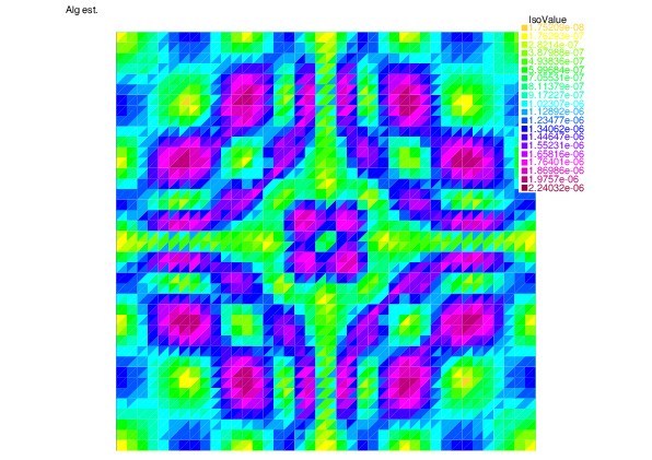 | |
| Algebraic error | Algebraic estimator |
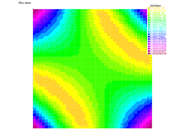 |
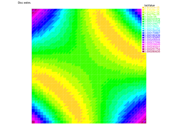 | |
| Discretization error | Discretization estimator |
download the script: ASCLapalceI.edp
You can also download the optimized version ASCLapalceII.edp.
A result of the comparison between the two version can be shown as follows:
The non-optimized version
 we need the computation time = 6.2107
 The number of iterations we need is = 100
 we need the computation time = 1.51902
 The number of iterations we need is = 100
return to main page