A posteriori error estimation based on the equilibrated flux recontruction
The Laplace problem
Let $\Omega\subset \mathbb{R}^2$ be an open bounded polygonal domain with the boundary donoted by $\partial \Omega$. Let us consider here the Laplace equation: for $f\in L^2(\Omega)$, find $u: \Omega \rightarrow \mathbb{R}$ such that $$\begin{align} -\Delta u = f &\qquad \mbox{ in }\Omega, \\ u = 0 & \qquad \mbox{ on } \partial\Omega. \end{align} $$ The variational formulation is defined by: Find $u\in H^1_0(\Omega)$ such that $$ (\nabla u, \nabla v) = (f,v) \qquad \forall v\in H^1_0(\Omega). $$ We denote by $\mathcal{T}_h$ the mesh used in the following. $\mathcal{T}_h$ is a simplicial partition of the polytope $\Omega$, i.e. $\cup_{K\in\mathcal{T}_h} \overline{K} = \overline{\Omega}$, any $K\in\mathcal{T}_h$ is a closed simplex (a triangle in 2D), and the intersection of two different simplices is either empty (a vertex, an edge in 2D).
Here we consider the computational domain as a square, with an uniform mesh. The number of the node on each edge is denoted by numnode.
// define the mesh
int numnode = 80;
mesh Th = square(numnode,numnode);
// functional space for solution
fespace Vh(Th,P1);
// boundary condition
func gd=x*(x-1)*y*(y-1);

func f = -2*(x*x+y*y)+2*(x+y);

// variational formulation
varf a(uh,vh)=int2d(Th)(Grad(uh)'*Grad(vh)) + int2d(Th)(f*vh) + on(1,2,3,4,uh=gd);

// solve the laplace problem exactly
matrix A=a(Vh,Vh,solver=CG);
real[int] b=a(0,Vh);
uh[]=A^-1*b;
To obtain these equilibrated flux, we need to solve the local mixed finite element problem by the following four steps.
1) we construct the "patches" associated to each node in the mesh.
mesh ThaI=Th;
mesh[int] Tha(Th.nv);
matrix[int] Aa(Th.nv);


fespace Pa(ThaI,P1dc);
for(int i=0; i < Th.nv; ++i)
{
    phia[][i]=1; // phia
    Tha[i] = trunc (Th, phia > 0,label=10);
    if (Th(i).label==0) Tha[i]=change(Tha[i],flabel=10);
    phia[][i]=0; // phia
}
2) For the local problem, we need to construct the matrix
fespace VPa(ThaI,[RT1,P1dc]);

real epsregua = numnode*numnode*1e-10;   //regularization for local problems

for( int i=0; i < Th.nv ;++i)
{
//  to bluild the basic function
    phia[][i]=1; // phia
    ThaI = Tha[i];
    VPa [s1,s2,ra],[v1,v2,q];
    //matrix
    varf a([s1,s2,ra],[v1,v2,q]) = int2d(ThaI)( [s1,s2]'*[v1,v2] - ra*Div(v1,v2) - Div(s1,s2)*q - epsregua*ra*q )+ on(10, s1=0,s2=0);
    matrix Art=a(VPa,VPa);
    Aa[i]= Art;
    set(Aa[i],solver=sparsesolver);
    phia[][i]=0;
}
3) We need also the right-hand-side of the local problems, and we solve them.
//for loop computing right hand side and solve the local problems
fespace Pa(ThaI,P1dc);
fespace VRT(Th,RT1);

VRT [sigma1,sigma2]=[0,0];
for(int i=0; i < Th.nv ;++i)
{
    phia[][i]=1; // phia
    ThaI = Tha[i];
    VPa [s1,s2,ra],[v1,v2,q];
    //right hand side
    varf l([uv1,uv2,uq],[v1,v2,q]) = int2d(ThaI)( - phia*(Grad(uh)'*[v1,v2] + f*q) + Grad(phia)'*Grad(uh)*q)
				    + on(10,uv1 = 0, uv2 = 0);
    VPa [F,F1,F2] ; F[] = l(0,VPa);
    Fa[i].resize(F[].n);
    Fa[i]=F[];
    s1[] = Aa[i]^-1*Fa[i];
    real[int] so(s1[].n);
    so=sigma1[](I[i]);
    s1[]= s1[].*epsI[i];
    s1[] += so;
    sigma1[](I[i]) = s1[];
    phia[][i]=0;
}
4) with this equilibrated flux, we can compute our estimator
// computation for the estimator

varf indicatorEtaDisc(unused,chiK) = int2d(Th)(chiK*( (Grad(uh) + [sigma1,sigma2]) '* (Grad(uh) + [sigma1,sigma2])  ))
	     + int2d(Th)(chiK*(hTriangle*hTriangle/pi/pi* (f-Div(sigma1,sigma2))*(f-Div(sigma1,sigma2)) ));
Wh mapEtaDisc;
mapEtaDisc[]=indicatorEtaDisc(0,Wh);
real GlobalEstimator=sqrt(mapEtaDisc[].sum);
mapEtaDisc=sqrt(mapEtaDisc);
plot(mapEtaDisc,  ps="MapDiscretisationEstimator.eps",value=1, fill=1,cmm="DiscretizationEstimator");
In order to showcase the performance of the estimator, we consider an example with an analytic solution,
// case with an analytic solution, and its derivatives [dx(u),dy(u)]
func uExact = x*(x-1)*y*(y-1);
func dxuExact=(2*x-1)*y*(y-1);
func dyuExact=(2*y-1)*x*(x-1);
// boundary condition
func gd=x*(x-1)*y*(y-1);
func f = -2*(x*x+y*y)+2*(x+y);
We compute the exact error (discretization error)
// computation for the exact error and map of error distribution
fespace Wh(Th,P0); // constant in each element
varf indicatorErrorTotal(unused,chiK) = int2d(Th)(chiK*((Grad(uh)-[dxduExact,dyduExact])'*(Grad(uh)-[dxduExact,dyduExact])));
Wh mapErrorTotal;
mapErrorTotal[]=indicatorErrorTotal(0,Wh);
real GlobalError=sqrt(mapErrorTotal[].sum);
mapErrorTotal=sqrt(mapErrorTotal);
plot(mapErrorTotal, ps="MapDiscretisationError.eps",value=1, fill=1,cmm="DiscretisationError");
-
We show here the analytic solution ($u$) and the solution obtained by the finite element method ($u_h$)
 |
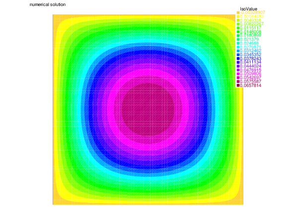 | |
| Analytic solution $u$ | Numerical solution $u_h$ |
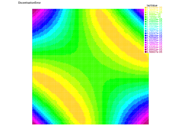
as well as the distribution of the discretization error $\|u-u_h\|_K$ and the estimator $\eta_{{\rm F},K}+\eta_{{\rm R},K}$
 |
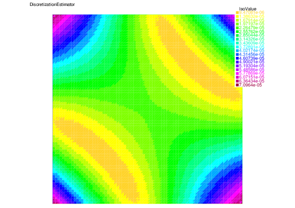 | |
| Discretization error | Discretization estimator |
With five levels of uniform mesh refinement, the effectivity index (the ratio between the total estimator and the total error) is given as follows:
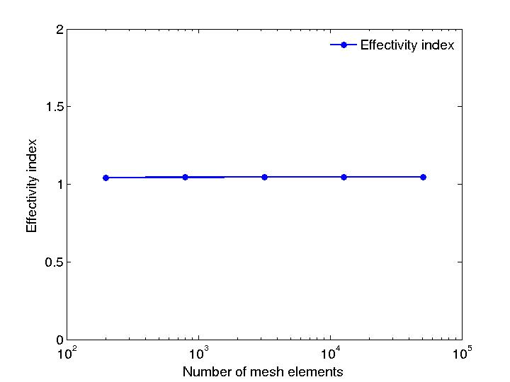 | |
| Effectivity index |
download the script: LaplaceVersionI.edp or return to main page