Implementation of a posteriori estimator with Freefem++

A posteriori estimator distinguishing different error components and adaptive stopping criteria

The $p$-Laplacian problem: distinguishing the algebraic, discretization, and linearization error components

Here, we will show the implementation work about the error estimator for the $p$-Laplacian problem which can distinguish the different error component in the computation, respectively the algebraic, linearization, and discretization error parts.

In the following, only some extractions of the full script will be shown to help understand the implementation work. You can download the full script at the end of this page.

We define the mesh, as for the $p$-Laplacian problem, we chose $p=10$ for example, so $q$ is given by $q=p/(p-1)$.

// definition of mesh
int numnode=30;       
mesh Th=square(numnode,numnode);
plot(Th,cmm="mesh",ps="mesh.eps");

// for the P-laplacian problem, we have 1/p+1/q=1
//  the value for p and q. p/2 and q/2
//real numberp=10;                  // value of p
real numberp=9;                 
real numberpdiv2=numberp/2;       // value of p/2
real numberq=numberp/(numberp-1); // value of q  
real numberqdiv2=numberq/2;       // value of q/2

We use an analytic solution to test the performance of the adaptive inexact Newton method

// Data for given problem: exact solution
// case for p!=2
func uExact = 1.0/numberq* ((0.5)^numberq-sqrt((x-0.5)^2+(y-0.5)^2)^numberq);             // in the normal case
func dxuExact = -0.5*((x-0.5)^2+(y-0.5)^2)^(numberqdiv2-1)*(2*x-1);
func dyuExact = -0.5*((x-0.5)^2+(y-0.5)^2)^(numberqdiv2-1)*(2*y-1);
func f=2;

We begin with an initial solution which is not far away from the exact solution, to do this, we add some oscillations by the parameters mu and lamda:

// to make an initial solution with some oscillation: lamda et mu
real lamda = 1, mu = 0.5;

The classic Newton method to solve the $p$-laplacian problem is given by:


uhk = uExact*(1+4*lamda*x*(x-1)*y*(y-1));    // initial soluton which is close to the exact solution
func int SolverExactLinearCG()
{
    
    varf VarfLaplacien(uh,vh)= int2d(Th)(((numberp-1)*(sqrt(Grad(uhk)'*Grad(uhk)))^(numberp-2))*Grad(uh)'*Grad(vh))
			      +int2d(Th)(f*vh+((numberp-2)*(sqrt(Grad(uhk)'*Grad(uhk)))^(numberp-2))*Grad(uhk)'*Grad(vh))
			      +on(1,2,3,4,uh=uExact);
    varf VarfBC1(uh,vh)=on(1,2,3,4,uh=1);				    
    matrix A=VarfLaplacien(Uh,Uh,tgv=-1,solver=GMRES);

    real[int] b=VarfLaplacien(0,Uh,tgv=-1);
    real[int] BC1=VarfBC1(0,Uh,tgv=-1);
    
    real epsgc=1e-10;
    func real[int] DJ(real[int] &u)
    {
	real[int] Au=A*u;
	return Au; 
    }
   
    int NumLinearization=0;		
    real eps1=1e-8;
    
    for (int k=1; k<=1000; k++)
    {	
	NumLinearization++;   
	
	A=VarfLaplacien(Uh,Uh,tgv=-1,solver=GMRES);
	b=VarfLaplacien(0,Uh,tgv=-1);     		    
	uh[] = BC1 ? b : uhk[]; 
	
	LinearCG(DJ,uh[],b,veps=epsgc,nbiter=1000,verbosity=nbverbosity);	
	epsgc=-abs(epsgc);

	Uh udiff=uh-uhk;
	if ((abs(udiff[].max) < eps1)||(abs(numberp-2) < eps1)) break;
	uhk=uh;
    }				 
    udisc=uh;
}			 
SolverExactLinearCG();

We denote the different types of solution by:

Uh uh;        // obtained solution at the (precedent+nu) step
Uh uhk;      // obtained solution at the LAST Newton linearization step by adaptive inexact method
Uh udisc;    // obtained solution by a exact algebraic solver and exact Newton linearization
Uh uhinfiny; // obtained solution by a exact algebraic solver at each Newton linearization
Uh uhp;      // obtained solution at the precedent step

The functions to compute different types of error

//  Computation of Total error:              uExact -- uhp
func real ComputeErrorTotal(int setValuePlot)

//  Computation of Discretization error:     uExact -- uDisc
func real ComputeErrorDisc(int setValuePlot)

//  Computation of Algebraic error:          uDisc - uhinfiny 
func real ComputeErrorLin(int setValuePlot)

//  Computation of Linearization error:      uhinfiny --uhp
func real ComputeErrorAlg(int setValuePlot)

Adaptive inexact Newton method to solve the $p$-Laplacian problem

uhk = uExact*(1+4*lamda*x*(x-1)*y*(y-1));    // initiale soluton which is close to the exact solution
func int SolverInexactAdaptiveLinearCG()
{
  
  
    varf VarfLaplacien(uh,vh)= int2d(Th)(((numberp-1)*(sqrt(Grad(uhk)'*Grad(uhk)))^(numberp-2))*Grad(uh)'*Grad(vh))
			      +int2d(Th)(f*vh) + int2d(Th)(((numberp-2)*(sqrt(Grad(uhk)'*Grad(uhk)))^(numberp-2))*Grad(uhk)'*Grad(vh))
			      +on(1,2,3,4,uh=uExact);
    varf VarfBC1(uh,vh)=on(1,2,3,4,uh=1);				    
    matrix A=VarfLaplacien(Uh,Uh,tgv=-1,solver=GMRES);
    set(A,solver=CG);
    real[int] b=VarfLaplacien(0,Uh,tgv=-1);
    real[int] BC1=VarfBC1(0,Uh,tgv=-1);
    
    
    func real[int] DJ(real[int] &u)
    {
	real[int] Au=A*u;
	return Au; 
    }
   
   
    // main part for the solving 
    NumLinearization=0;		
    real epsgc=1e-10;
    
    for (int k=1; k<=1000; k++)
    {	
	NumLinearization++;   
	A=VarfLaplacien(Uh,Uh,tgv=-1,solver=GMRES);

	b=VarfLaplacien(0,Uh,tgv=-1);     		    
	uh[] = BC1 ? b : uhk[]; 	
	LinearCG(DJ,uh[],b,eps=eps1,nbiter=1000,verbosity=nbverbosity,stop=stop);	

	if(CritereArret == 3) break;	
	uhk=uh;
    }				 
}	

SolverInexactAdaptiveLinearCG();

The adaptive stopping criteria is defined in the "stop" function, which is given by:

    func bool stop(int iter, real[int] u, real[int] g)
    {
	CritereArret = 10;
	if (iter%nu==0 && iter > 1){
		sigma1=(sqrt(Grad(uh)'*Grad(uh)))^(numberp-2)*dx(uh);
		sigma2=(sqrt(Grad(uh)'*Grad(uh)))^(numberp-2)*dy(uh);
		sigmak1=(numberp-1)*(sqrt( Grad(uhk)'*Grad(uhk)))^(numberp-2)*dx(uh)-(numberp-2)*(sqrt(Grad(uhk)'*Grad(uhk)))^(numberp-2)*dx(uhk);
		sigmak2=(numberp-1)*(sqrt( Grad(uhk)'*Grad(uhk)))^(numberp-2)*dy(uh)-(numberp-2)*(sqrt(Grad(uhk)'*Grad(uhk)))^(numberp-2)*dy(uhk);			
		CritereArret=ComputeEstimator(iter);	
		if (CritereArret == 2 || CritereArret == 3) return 1;
	}
	return 0;
    }

Here, as sigma1,sigma2, sigmak1,sigmak2 are always constant in each element due to the considered finite element, we compute it in advance in order to reduce the computational time. These constants will be used in the local problem for the equilibrated flux reconstruction.

The function ComputeEstimator is the main part, which correspond the adaptive inexact Newton algorithm and the stopping criterion.


    func int ComputeEstimator(int numiterCG)
    {
	if (numiterCG==nu){ 			
	    RHSdplusl();  // compute d+l
	    RHSd();	  // compute d
	    uhp=uh;   	  // in each Newton linearization, we begin from uh
	    [d1p,d2p]=[d1,d2];
	    [dplusl1p,dplusl2p]=[dplusl1,dplusl2];
		
	    real etaDisc=ComputeEtaDisc(0);
	    real etaLin=ComputeEtaLin(0);
	    etaDiscSave=etaDisc;
	    etaLinSave=etaLin;
	}else{
	    RHSdplusl();  //compute d+l
	    RHSd();	  //compute d		
	    real etaRem=ComputeEtaRem(0);
	    real etaAlg=ComputeEtaAlg(0);
	    real maxError1=max(etaDiscSave,etaLinSave);
	    real maxError2=max(maxError1,etaAlg);
	    if (etaRem>GammaRem*maxError2)
	    {
		return 1;
	    }else{
		if (etaAlg>GammaAlg*maxError1){
  		    uhp=uh;
		    [d1p,d2p]=[d1,d2];
		    [dplusl1p,dplusl2p]=[dplusl1,dplusl2];	
		    real etaDisc=ComputeEtaDisc(0);
		    real etaLin=ComputeEtaLin(0);	
		    etaDiscSave=etaDisc;
		    etaLinSave=etaLin;
		    return 1;
		}else{
		    if (etaLinSave<=GammaLin*etaDiscSave){
			return 3;
		    }
		    uhk=uhp;
		    return 2;
		}
	    }
	}
    }

We have four functions to compute the different estimators, respectively:


func real ComputeEtaDisc(int setValuePlot)
{  
  real etaDisc;
    if (setValuePlot)
    {
//	varf indicatoretaDisc(unused,chiK) = int2d(Th)(chiK*(((sqrt(Grad(uh)'*Grad(uh))^(numberp-2)*Grad(uh)+[d1,d2])'* (sqrt(Grad(uh)'*Grad(uh))^(numberp-2)*Grad(uh)+[d1,d2]))^numberqdiv2));
	varf indicatoretaDisc(unused,chiK) = int2d(Th)(chiK*(((sqrt(Grad(uhp)'*Grad(uhp))^(numberp-2)*Grad(uhp)+[d1,d2])'* (sqrt(Grad(uhp)'*Grad(uhp))^(numberp-2)*Grad(uhp)+[d1,d2]))^numberqdiv2));
	Wh mapetaDisc;
	mapetaDisc[]=indicatoretaDisc(0,Wh);
	etaDisc=2^(1.0/numberp)*(mapetaDisc[].sum)^(1.0/numberq);
	mapetaDisc=2^(1.0/numberp)*(mapetaDisc)^(1.0/numberq);
	plot(mapetaDisc, ps="MapDiscEstimator.eps",value=1, fill=1,cmm="DiscretizationEstimator");
    }else
    {
	etaDisc=int2d(Th)(((sqrt(Grad(uhp)'*Grad(uhp))^(numberp-2)*Grad(uhp)+[d1p,d2p])'* (sqrt(Grad(uhp)'*Grad(uhp))^(numberp-2)*Grad(uhp)+[d1p,d2p]))^numberqdiv2);	
	etaDisc=2^(1.0/numberp)*etaDisc^(1.0/numberq);
    }
    return etaDisc;
}



func real ComputeEtaAlg(int setValuePlot)
{  
  real etaAlg;
    if (setValuePlot)
    {
	varf indicatoretaAlg(unused,chiK) = int2d(Th)(chiK*( ( ([dplusl1,dplusl2]-[dplusl1p,dplusl2p])'*([dplusl1,dplusl2]-[dplusl1p,dplusl2p]) )^numberqdiv2 ));
	Wh mapetaAlg;
	mapetaAlg[]=indicatoretaAlg(0,Wh);
	etaAlg=(mapetaAlg[].sum)^(1.0/numberq);
	mapetaAlg=(mapetaAlg)^(1.0/numberq);
	plot(mapetaAlg, ps="MapAlgebraicEstimator.eps",value=1, fill=1,cmm="AlgebraicEstimator");
    }else
    {
	etaAlg=int2d(Th)( ( ([dplusl1,dplusl2]-[dplusl1p,dplusl2p])'*([dplusl1,dplusl2]-[dplusl1p,dplusl2p]) )^numberqdiv2 );	
	etaAlg=etaAlg^(1.0/numberq);
    }
    return etaAlg;
}

			

func real ComputeEtaLin(int setValuePlot)
{  
  real etaLin;
    if (setValuePlot)
    {
	varf indicatoretaLin(unused,chiK) = int2d(Th)(chiK*(( ([dplusl1p,dplusl2p]-[d1p,d2p])'*([dplusl1p,dplusl2p]-[d1p,d2p]))^numberqdiv2));
	Wh mapetaLin;
	mapetaLin[]=indicatoretaLin(0,Wh);
	etaLin=(mapetaLin[].sum)^(1.0/numberq);
	mapetaLin=(mapetaLin)^(1.0/numberq);
	plot(mapetaLin, ps="MapLinearizationEstimator.eps",value=1, fill=1,cmm="LinearizationEstimator");
    }else
    {
	etaLin=int2d(Th)(( ([dplusl1p,dplusl2p]-[d1p,d2p])'*([dplusl1p,dplusl2p]-[d1p,d2p]))^numberqdiv2 );	
	etaLin=etaLin^(1.0/numberq);
    }
    return etaLin;
}


    func real ComputeEtaRem(int setValuePlot)
    {
	real[int] rh(Th.nt);
	real[int] rhK(Th.nt);	//vector rh multiply area of their triangle
	rh = 0.;
	for(int i=0; i < Th.nt; i++) 
	{
	    for(int j=0; j < 3; j++) 
	    {
		int indv = Th[i][j];
		rh[i] += (Ra[indv]/Tha[indv].area);
	    }
	    rhK[i] = rh[i]*(Th[i].area)^(2.0/numberq);
	} 
	real etaRem = (diameterArea * sqrt(rh'*rhK));  
	return etaRem;	
    }

Now, the point is how to construct the equilibrated flux, as denoted by $d+l$ and $d$ at $i$th step in the algebraic solver, as well as at $(i+nu)$-th step. In my script, I denoted them by

fespace Vh(Th,RT1);  // Raviart-Thomas space
// valeur de d et d_precedent
Vh [d1,d2] = [0,0];
Vh [d1p,d2p] = [0,0];
// valeur de d+l et d+l_precedent
Vh [dplusl1,dplusl2] = [0,0];
Vh [dplusl1p,dplusl2p] = [0,0];

To obtain these equilibrated flux, we need to solve the local mixed finite element problem.
Firstly, we construct the "patches" associated to each node in the mesh.

    fespace Pa(ThaI,P1dc);
    for(int i=0; i < Th.nv; ++i)
    {
	phia[][i]=1; // phia 
	Tha[i] = trunc (Th, phia > 0,label=10);
	if (Th(i).label==0) Tha[i]=change(Tha[i],flabel=10);  
	phia[][i]=0; // phia 
    }

For the local problems, we have the same matrix during the algorithm, so we prepare it in advance


  real epsregua = numnode*numnode*1e-8;  //regularisation term to ensure the uniqueness of the solution of the local problem

  matrix[int] Aa(Th.nv);

  func int globalMatrix(matrix[int] & Aa) 
    {
	for( int i=0; i < Th.nv ;++i) 
	{
		phia[][i]=1; // phia 
		ThaI = Tha[i];
		VPa [dIa1,dIa2,qa],[v1,v2,phih];
	 
		varf Varflocala([dIa1,dIa2,qa],[v1,v2,phih]) = 
			int2d(ThaI)( [dIa1,dIa2]'*[v1,v2] - qa*Div(v1,v2) - Div(dIa1,dIa2)*phih - epsregua*qa*phih )
			+ on(10, dIa1=0,dIa2=0);
		matrix Art=Varflocala(VPa,VPa);	
		Aa[i]= Art; 
		set(Aa[i],solver=sparsesolver); 			
		phia[][i]=0;
	}
    }
    globalMatrix(Aa);

Here we add one regularization term as $-\int_{ThaI} epsregua*qa*phih$ to ensure the average value of $qa$ is 0.

Eachtime we do the estimation, we need to solve the two local problems, respectively for $d$ and $d+l$, as the matrix is same during the inexact Newton algorithm, only the right-hand-side change, we here call the functions RHSd() and RHSdplusl().
Attention, here we can do some optimizations for the code, as shown for the laplace problem. i.e. we can prepare a table of matrix associated to the RHS in advance, as well as the computational part for each estimator.


   func int RHSd() 
    {
	Vh [d11,d22]=[0,0];
	int indv=0;	
	// boucle pour calculer le residu Rabas dans le probleme local d
	for(int i=0; i < Th.nv; i++) {
		phia[][i]=1; 
		ThaI = Tha[i];
		Rabas[i] = int2d(ThaI)(f'*phia-(sqrt(Grad(uh)'*Grad(uh)))^(numberp-2)*(Grad(uh)'*Grad(phia)));
		phia[][i]=0;
	}
	//set value of Rabas to zero for vertices lie on the boundary
	indv = 0;
	for(int i=0; i < Th.nbe; i++) {
	    for(int j=0; j < 2; j++) {
		indv = Th.be(i)[j];
		Rabas[indv] = 0.;
	    }
	}
	for(int i=0; i < Th.nv ;++i) 
	{
		phia[][i]=1; 
		ThaI = Tha[i];	
		Pa Chia =1; 
		VPa [d1tmp,d2tmp,qa],[v1,v2,phih];			
		
		varf l([uv1,uv2,qa],[v1,v2,phih]) = -int2d(ThaI)( phia*(([sigma1,sigma2])'*[v1,v2] + f*phih )
					  -Grad(phia)'*[sigma1,sigma2]*phih - Rabas[i]*phih/ThaI.area)
			+ on(10,uv1 = 0, uv2 = 0);
		VPa [F,F1,F2] ; 
		F[] = l(0,VPa);
		Fa[i].resize(F[].n);
		Fa[i]=F[];
		d1tmp[] = Aa[i]^-1*Fa[i];		
		real[int] so(d1tmp[].n);
		so=d11[](I[i]);
		d1tmp[]= d1tmp[].*epsI[i];
		d1tmp[] += so;
		d11[](I[i]) = d1tmp[];		
		phia[][i]=0;
	}	
	[d1, d2]=[d11,d22];
	return 1;
    }

 func int RHSdplusl() 
    {
	Vh [dplusl11,dplusl22]=[0,0];
	int indv=0;
	//for loop computing vector Ra
	for(int i=0; i < Th.nv; i++) {
		phia[][i]=1; 
		ThaI = Tha[i];
		Ra[i] = int2d(ThaI)(f'*phia
		-(numberp-1)* (sqrt( Grad(uhk)'*Grad(uhk)))^(numberp-2)*(Grad(uh)'*Grad(phia))
		+ (numberp-2)*(sqrt(Grad(uhk)'*Grad(uhk)))^(numberp-2)*(Grad(uhk)'*Grad(phia)));				
		phia[][i]=0;
	}
	//set value of Ra to zero for vertices lie on the boundary
	indv = 0;
	for(int i=0; i < Th.nbe; i++) 
	{
	    for(int j=0; j < 2; j++) 
	    {
		indv = Th.be(i)[j];			
		Ra[indv] = 0.;
	    }
	}
	for(int i=0; i < Th.nv ;++i) 
	{
	    phia[][i]=1; 
	    ThaI = Tha[i];	
	    Pa Chia =1; 
	    VPa [dplusl1tmp,dplusl2tmp,qa],[v1,v2,phih];			
 	    varf l([uv1,uv2,qa],[v1,v2,phih]) = -int2d(ThaI)( phia*(([sigmak1,sigmak2])'   *[v1,v2] + f*phih)
 			-Grad(phia)'*[sigmak1,sigmak2]*phih - Ra[i]*phih/ThaI.area)
			+ on(10,uv1 = 0, uv2 = 0);
	    VPa [F,F1,F2] ; 
	    F[] = l(0,VPa);
	    Fa[i].resize(F[].n);
	    Fa[i]=F[]; 
	    dplusl1tmp[] = Aa[i]^-1*Fa[i];		
	    real[int] so(dplusl1tmp[].n);
	    so=dplusl11[](I[i]);
	    dplusl1tmp[]= dplusl1tmp[].*epsI[i];
	    dplusl1tmp[] += so;
	    dplusl11[](I[i]) = dplusl1tmp[];		
	    phia[][i]=0;
	}	
	[dplusl1,dplusl2]=[dplusl11,dplusl22];
	return 1;
    }

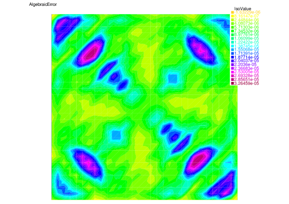
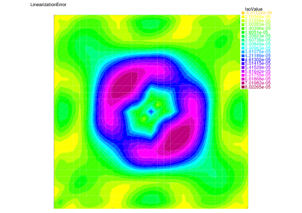
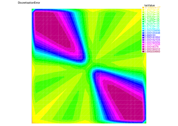
We see that for each error component: discretization, algebraic, and linearization errors, the overall error distributions are very well predicted by the corresponding estimators.


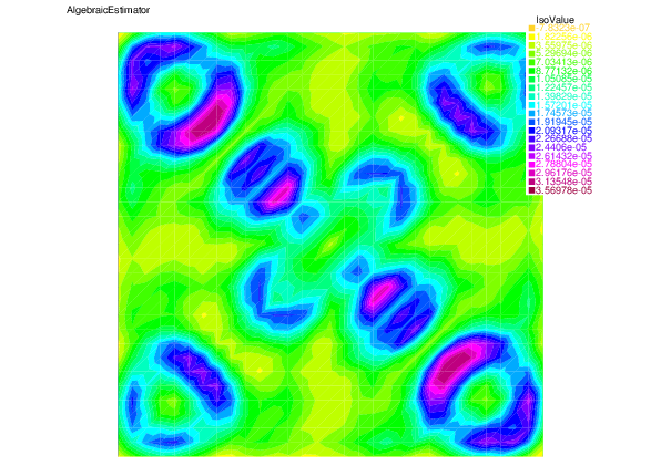Algebraic error	Algebraic estimator


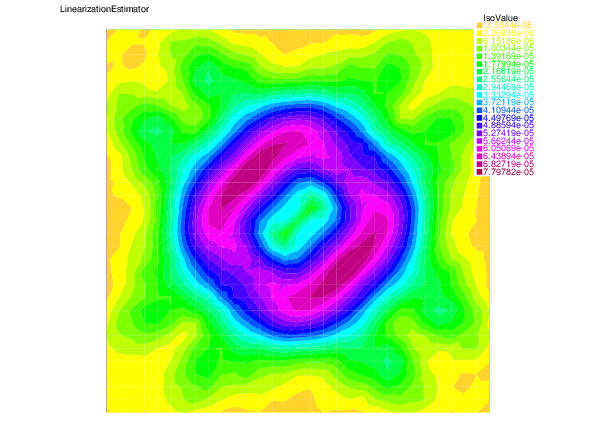Linearization error	Linearization estimator


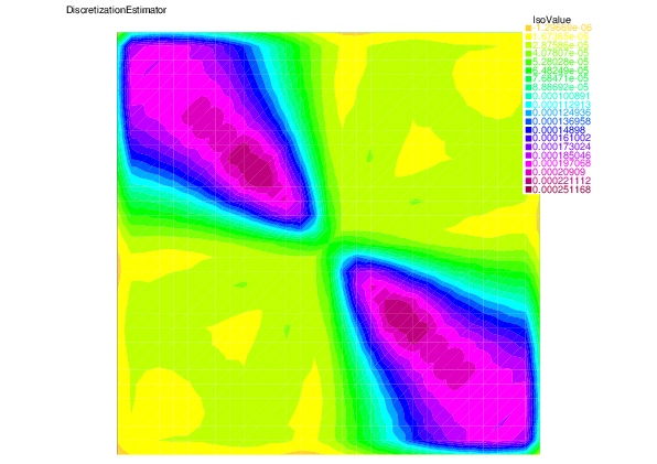Discretization error	Discretization estimator

download the script: ASCpLapalceI.edp or return to main page