A posteriori estimator distinguishing different error components and adaptive stopping criteria
The Stokes problem with Uzawa algorithm: distinguish the algebraic, discretization, and the Uzawa error components
In the following, we will show an extraction of the numerical part in our article. More details can be found in our pre-print here
As shown in the exact Uzawa algorithm for the Stokes problem, we use two loops in the computation. One loop for the Uzawa iteration which updates the pressure $p$, and another loop in the algebraic solver for solving the velocity $\mathbf{u}$ at each Uzawa iteration.
As the mesh is fixed, the question is "DO WE REALLY NEED SO MANY ITERATIONS IN THE UZAWA ALGORITHM AND THE ALGEBRAIC SOLVER?"
Here, we will show you the implementation work about the error estimator which can distinguish the different error components in the computation, respectively the algebraic, Uzawa, and discretization error components. With these estimators, we can define an adaptive version of the inexact Uzawa algorithm, that means, we stop the Uzawa iteration and the algebraic solver iteration when the Uzawa error component, respectively the algebraic solver error component, do not have a significant influence on the total error.
We consider here the computational domain as $\Omega=(0,1)^2$, with homogeneous Dirichlet boundary conditions. The exact solution is given as follows with the value $\alpha=1$, \[\mathbf{u}= \left(\begin{array}{c} 2 x^2 y (x - 1)^2 (y - 1)^2 + x^2 y^2 (2 y - 2) (x - 1)^2\\ - 2 x y^2 (x - 1)^2 (y - 1)^2 - x^2 y^2 (2 x - 2) (y - 1)^2\\ \end{array}\right)\] and \[p=x+y-1.\] The volumetric force $\mathbf{f}$ is chosen accordingly.
To showcase the performance of our algorithm, we consider here three different approaches, respectively the exact Uzawa algorithm, the inexact Uzawa algorithm, and our adaptive inexact Uzawa algorithm:
Exact Uzawa algorithm
func real ExactCG(int nn)
{
    p=0;
    real epsgc= 1e-10;

    // Uzawa iteration
    int inumOuter=0;
    while(inumOuter<10000){  //to be changed after

  	b1[]=Bt*p[];  	b1[]+=F;   // second member for problem  Au=Btu+F
	b1[]= BC ? F : b1[];
	u1[]= BC ? F :  u1[];

	LinearCG(DJ,u1[],b1[],veps=epsgc,nbiter=2000,verbosity=0);
	epsgc=-abs(epsgc);

	real[int] Bu1=B*u1[];
	Bu1*=alpha;
	real normBu1=sqrt(Bu1'*Bu1);
	if (normBu1<1e-10) break;

	// update for p
	real[int] ptemp(p[].n);
	ptemp=C^-1*Bu1;  // C p^{k+1}=C p^{k} - alpha Bu
	p[]-=ptemp;
	p[]-=int2d(Th)(p)/AreaDomain;
	inumOuter++;
}
	ph=p;
	[uh1,uh2]=[u1,u2];     // save the solution of exact uzawa method
}
Inexact Uzawa algorithm
func bool stopCGInex(int iter, real[int] u, real[int] g)
{
    real normg=sqrt(g'*g);
    if (normg<=tau*normBu1){
	numIteInner[inumOuter]=iter+1;
	return 1;
    }
    return 0;
}

    while(inumOuter<2000){  //to be changed after
        numIteInner.resize(inumOuter+1);
	stopcriteria=0;


	b1[]=Bt*p[];  	b1[]+=F;   // second member for problem  Au=Btu+F
	b1[]= BC ? F : b1[];
	u1[]= BC? F: u1[];
	LinearCG(DJ,u1[],b1[],eps=1e-6,nbiter=1000,verbosity=0,stop=stopCGInex);

	real[int] Bu1=B*u1[];
	Bu1*=alpha;
	normBu1=sqrt(Bu1'*Bu1);
	inumOuter++;
	real[int] ptemp(p[].n);
	ptemp=C^-1*Bu1;  // C p^{k+1}=C p^{k} - alpha Bu
	p[]-=ptemp;
	p[]-=int2d(Th)(p)/AreaDomain;

 	real normdiffp=int2d(Th)((p-pp)'*(p-pp));
 	normdiffp=sqrt(normdiffp);
 	if (normdiffp<1e-8) break;
 	pp=p;
    }
}
Adaptive inexact Uzawa algorithm
func bool stop(int iter, real[int] u, real[int] g)
{
  if (iter%nu==0 && iter>0){
      stopcriteria=estimation(iter);
  }
  if (stopcriteria>0){
      numIteInner.resize(inumOuter+1);
      numIteInner[inumOuter]=iter;
      return 1;
  }
  return 0;
}


real epsgc= 1e-10;
usave1[]=0;
while(inumOuter<1000){  //to be changed after
	stopcriteria=0;


	u1[]=usave1[];
	b1[]=Bt*p[];
	b1[]+=F;   // second member for problem  Au=Btu+F
	b1[]= BC ? F : b1[];
	u1[]= BC ? F: u1[];

	LinearCG(DJ,u1[],b1[],eps=1e-6,nbiter=1000,verbosity=0,stop=stop);

	real[int] Bu1=B*u1[];
	Bu1*=alpha;
	real normBu1=sqrt(Bu1'*Bu1);
	if (stopcriteria==2) break;
	inumOuter++;
	real[int] ptemp(p[].n);
	ptemp=C^-1*Bu1;  // C p^{k+1}=C p^{k} - alpha Bu
	p[]-=ptemp;
	p[]-=int2d(Th)(p)/AreaDomain;
}
The main part for our stopping criterion is given as follows:
func int estimation(int innernum)
{
	if (innernum==nu){
		RHSd();

		[d11p,d12p,d21p,d22p]=[d11,d12,d21,d22];
		[usave1,usave2]=[u1,u2];
		real etaDisc=   ComputeEtaDisc(0);
		real etaUzawa =   ComputeEtaUzawa(0);
		etaDiscSave=etaDisc;
		etaUzawaSave=etaUzawa;
	}else{
		RHSd();
 		real etaRem=ComputeEtaRem(0);
 		real etaAlg=ComputeEtaAlg(0);

		real maxError1=max(etaDiscSave,etaUzawaSave);
		real maxError2=max(maxError1,etaAlg);

		if (etaRem>GammaRem*etaAlg){
			return 0;
		}else{

			if (etaAlg>GammaAlg*maxError1){

			 	[d11p,d12p,d21p,d22p]=[d11,d12,d21,d22];
				[usave1,usave2]=[u1,u2];

 				real etaDisc= ComputeEtaDisc(0);
 				real etaDK= ComputeEtaDK(0);
 				real etaUzawa = ComputeEtaUzawa(0);
				etaDiscSave=etaDisc;
				etaUzawaSave=etaUzawa;
				return 0;
			}else{
				if (etaUzawaSave<=GammaUzawa*etaDiscSave){
					return 2;
				}
				[usave1,usave2]=[u1,u2];
				return 1;
			}
		}
	}
return 0;
}
We consider eight levels of uniform mesh refinement.
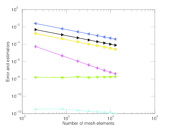
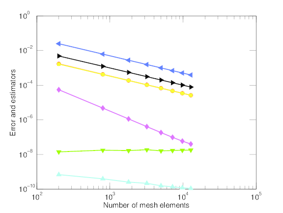
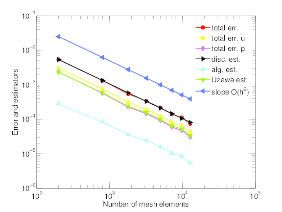
We present the total error and the various estimators as a function of the number of mesh elements. It can be seen that the three approaches yield almost indistinguishable value for the total error; in this smooth case, the convergence order is $O(h^2)$. For the exact and inexact Uzawa method, the estimators of Uzawa iterations take the values around $10^{-8}$, and the estimators of algebraic solver are much smaller in the exact case than in the inexact one. For the adaptive inexact method, we terminate the computation with much larger estimators for Uzawa iterations and algebraic solver iterations, just sufficient not to influence the total error. For all the three methods, the total estimators converge with the same speed as the total error.
 |
 |
 | |
| Exact Uzawa | Inexact Uzawar | Adaptive inexact Uzawar |
Error and estimators on uniformly refined meshes: exact, inexact, and adaptive inexact
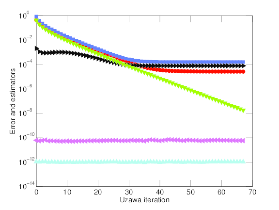
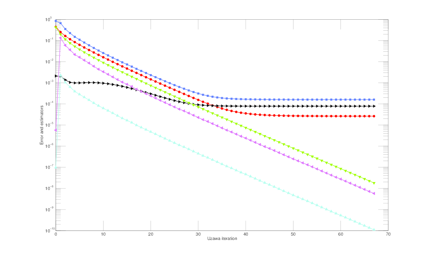
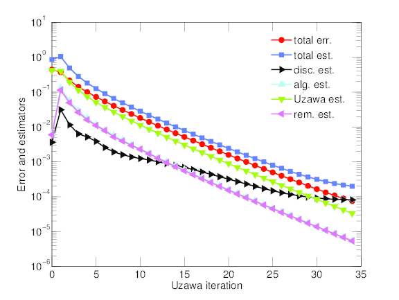
Now, we focus on the finest mesh, and displays the dependence of the total error and of the various estimators on the Uzawa iteration. The total error and the total estimator decrease rapidly for the first $30$-$40$ Uzawa iterations and then only very slowly, since therefrom the influence of the Uzawa iteration error gets negligible. This is precisely the point where our adaptive inexact Uzawa method stops, leading to an important economy of the Uzawa iterations used.
 |
 |
 | |
| Exact Uzawa | Inexact Uzawar | Adaptive inexact Uzawar |
Error and estimators as a function of Uzawa iterations: exact, inexact, and adaptive inexact
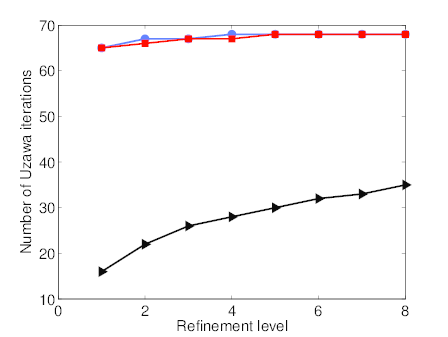
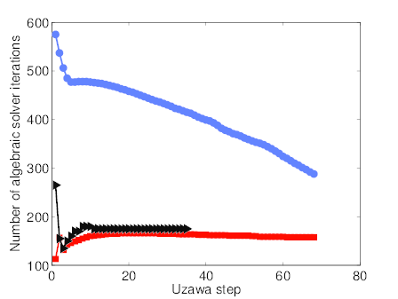
The overall performance of the three approaches is compared as follows. We present the number of Uzawa iterations as a function of the refinement level, the number of algebraic solver iterations as a function of Uzawa iteration on the last refined mesh, and the total number of algebraic solver iterations as a function of the refinement level. Concerning the total number of Uzawa iterations, the exact and inexact methods show no significant difference. The adaptive inexact method reduces this count by a factor bigger than two. Gratifyingly, the inexact and the adaptive inexact methods need almost the same number of CG iterations on each Uzawa step. In combination, the adaptive inexact method needs the smallest number of total algebraic solver iterations; on the eighth refined mesh, the three approaches need respectively 31499, 11162, and 6295 total algebraic solver iterations.
 |
 |
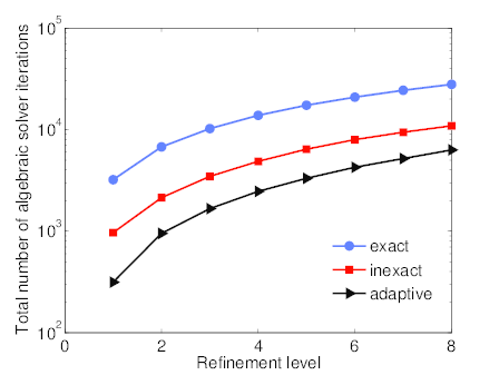 | |
| Number of Uzawa iterations per refinement level | Number of linear solver iterations per Uzawa step on the eighth-level mesh | Total number of linear solver iterations per refinement level |
Number of linear solver and Uzawa iterations
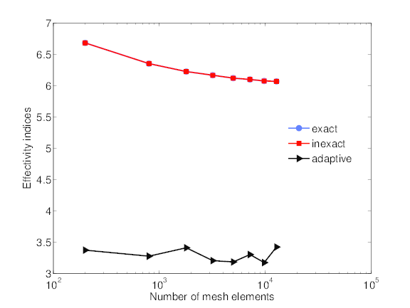
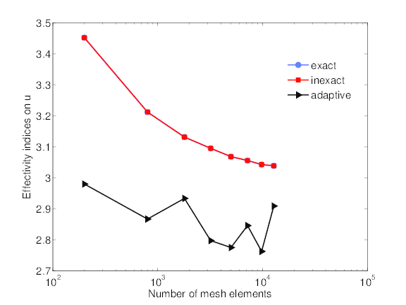
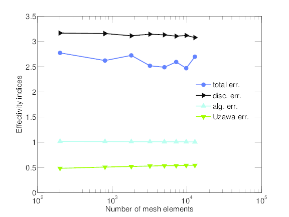
The total effectivity indices for the three approaches are presented in Figure~\ref{figure5}. There are computed as the ratio between the total estimator and the total error. We consider additionally the effectivity indices for the velocity and the pressure.
 |
 |
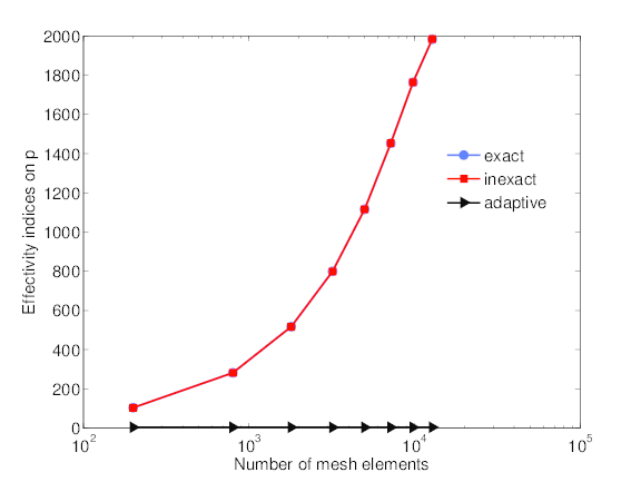 | |
| total effectivity index | effectivity index for the velocity | effectivity index for the pressure |
Effectivity indices
as well as the effectivity indices for each error component in the adaptive inexact algorithm
 |
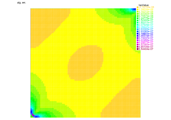
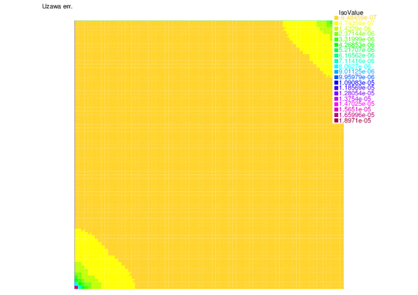
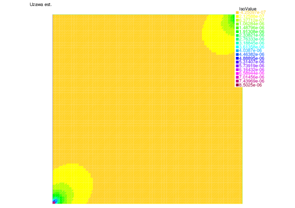
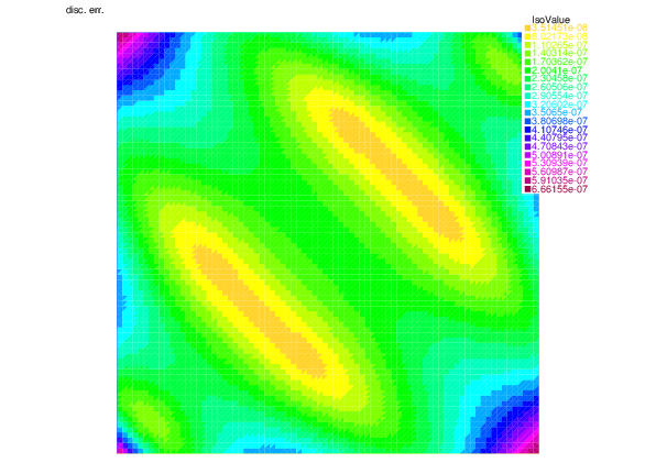
At last, we display the spatial distribution of the different error components (left) and of the corresponding estimators (right), on the eighth refined mesh. We can observe a nice match.
 |
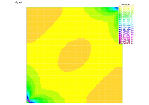 | |
| Algebraic error | Algebraic estimator |
 |
 | |
| Uzawa error | Uzawa estimator |
 |
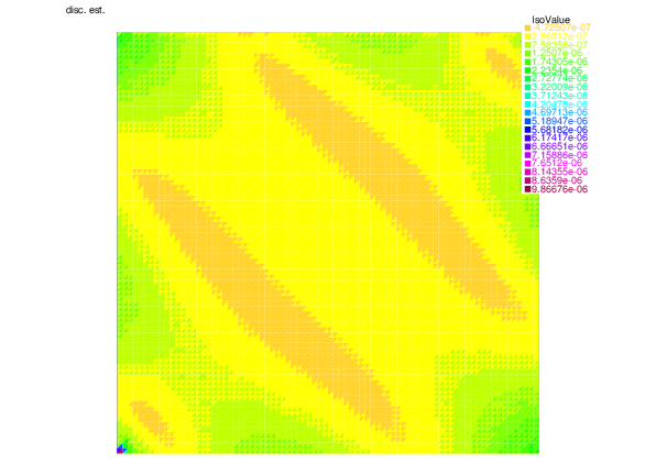 | |
| Discretization error | Discretization estimator |
return to main page