A posteriori error estimation based on the equilibrated flux reconstruction
The Stokes problem
Let $\Omega\subset \mathbb{R}^2$ be an open bounded polygonal domain with the boundary denoted by $\partial \Omega$. Let us consider here the steady linear Stokes model: let a source function $\mathbf{f}: \Omega \rightarrow \mathbb{R}^2$ (a vector here) be given. The Stokes problem consists in finding the velocity $\mathbf{u}: \Omega \rightarrow \mathbb{R}^2$ and the pressure $p: \Omega \rightarrow \mathbb{R}$ such that $$\begin{align} -\Delta \mathbf{u} + \nabla p = \mathbf{f} &\qquad \mbox{ in }\Omega, \\ \nabla \cdot \mathbf{u} = 0 & \qquad \mbox{ in }\Omega, \\ \mathbf{u} = \mathbf{0} & \qquad \mbox{ on } \partial\Omega. \end{align} $$ The variational formulation is defined by: Find $(\mathbf{u},p)\in [H^1_0(\Omega)]^2\times L^2_0(\Omega)$ such that $$\begin{align} (\nabla \mathbf{u}, \nabla \mathbf{v})-(\nabla \cdot \mathbf{v}, p) &= (\mathbf{f},\mathbf{v}) &\qquad \forall \mathbf{v}\in [H^1_0(\Omega)]^2,\\ (\nabla\cdot \mathbf{u}, q)&=0 &\qquad \forall q\in L^2_0(\Omega). \end{align} $$ We denote by $\mathcal{T}_h$ the mesh used in the following. $\mathcal{T}_h$ is a simplicial partition of the polytope $\Omega$, i.e. $\cup_{K\in\mathcal{T}_h} \overline{K} = \overline{\Omega}$, any $K\in\mathcal{T}_h$ is a closed simplex (a triangle in 2D), and the intersection of two different simplices is either empty (a vertex, an edge in 2D).
Here we consider the computational domain as a square, with an uniform mesh. The number of the node on each edge is denoted by numnode.
// mesh to define
int numnode=80;
mesh Th=square(numnode,numnode);
plot(Th,cmm="mesh",ps="mesh.eps");
real AreaDomain=Th.area;
We consider the Taylor-Hood family finite element, i.e. $\mathbb{P}_2$ for the velocity and $\mathbb{P}_1$ for the pressure.
fespace Uh(Th,[P2,P2]);  // fonction space for  u=(u1,u2)
Uh [u1,u2],[v1,v2];
fespace Ph(Th,P1);       // function space for p
Ph p;
We consider exact Uzawa algorithm to solve the Stokes problem (more details about the Uzawa algorithm can be found here (page 267)).
p=0;
real epsgc= 1e-10;
// Uzawa iteration
int inumOuter=0;
while(inumOuter<10000){  //to be changed after

  	b1[]=Bt*p[];  	b1[]+=F;   // second member for problem  Au=Btu+F
	b1[]= BC ? F : b1[];
	u1[]= BC? F: u1[];

	LinearCG(DJ,u1[],b1[],veps=epsgc,nbiter=2000,verbosity=0);
	epsgc=-abs(epsgc);

	real[int] Bu1=B*u1[];
	Bu1*=alpha;
	real normBu1=sqrt(Bu1'*Bu1);
	if (normBu1<1e-10) break;

	// update for p
	real[int] ptemp(p[].n);
	ptemp=C^-1*Bu1;  // C p^{k+1}=C p^{k} - alpha Bu
	p[]-=ptemp;
	p[]-=int2d(Th)(p)/AreaDomain;
	inumOuter++;
}
ph=p;
[uh1,uh2]=[u1,u2];     // save the solution of exact uzawa method
For $1\leq m \leq 2$, we denote $\mathbf{e}_m\in \mathbb{R}^2$ the canonical verctor. We call the equilibrated flux reconstruction any function $\sigma_h$ constructed from $\mathbf{u}_h$ which satisfies $\sigma_h\in [\mathbf{H}(\rm div,\Omega)]^2$, $$(\nabla\cdot \sigma_h, \mathbf{e}_i)_K= (\mathbf{f}, \mathbf{e}_i)_K, \qquad i=1,...2, \forall K\in \mathcal{T}_h$$
For any $K\in \mathcal{T}_h$, define the residual estimator by: $$ \eta_{{\rm R},K} := \frac{h_K}{\pi} \|\mathbf{f}+\nabla \cdot \sigma_h\|_K, $$ the flux estimator by $$ \eta_{{\rm F},K} := \|\nabla \mathbf{u}_h- p_h \mathbb{I} - \sigma_h\|_K. $$ and the divergence estimator by $$ \eta_{{\rm D},K} := \frac{\|\nabla \cdot\mathbf{u}_h\|_K}{\beta}. $$ Then we have $$ \|\nabla (u-u_h)\|^2 \leq \sum_{K\in \mathcal{T}_h} (\eta_{{\rm R},K}+\eta_{{\rm F},K} )^2 + \sum_{K\in \mathcal{T}_h} \eta_{{\rm D},K}^2 $$ and $$ \beta\|p-p_h\| \leq \left\{\sum_{K\in \mathcal{T}_h} (\eta_{{\rm R},K}+\eta_{{\rm F},K} )^2\right\}^{1/2} + \left\{\sum_{K\in \mathcal{T}_h} \eta_{{\rm D},K}^2\right\}^{1/2} $$
To construct the equilibrated flux, we should solve the local Neumann mixed finite element problem, some more technical details can be found here. Using this way of reconstruction, we can ensure the polynomial-degree-robustness of the estimator
To obtain these equilibrated flux, we need to solve the local mixed finite element problem by the following four steps.
1) we construct the "patches" associated to each node in the mesh.
mesh ThaI=Th;
mesh[int] Tha(Th.nv);
matrix[int] Aa(Th.nv);


fespace Pa(ThaI,P1dc);
{
    phia[][i]=1; // phia
    Tha[i] = trunc (Th, phia > 0,label=10);
    if (Th(i).label==0) Tha[i]=change(Tha[i],flabel=10);
    phia[][i]=0; // phia
}
2) For the local problem, we need to construct the matrix
fespace VPa(ThaI,[RT1,RT1,P1dc,P1dc]);
matrix[int] Aa(Th.nv);

real epsregua = numnode*numnode*1e-10;

for( int i=0; i < Th.nv ;i++)
{
	phia[][i]=1; // phia
	ThaI = Tha[i];
	VPa [d11t,d12t,d21t,d22t,qa1,qa2],[vh11,vh12,vh21,vh22,phih1,phih2];
	varf Varflocala([d11t,d12t,d21t,d22t,qa1,qa2],[vh11,vh12,vh21,vh22,phih1,phih2]) =
	int2d(ThaI)( [d11t,d12t,d21t,d22t]'*[vh11,vh12,vh21,vh22]
	+ (qa1*Div(vh11,vh12)+qa2*Div(vh21,vh22))
	+ (Div(d11t,d12t)*phih1+Div(d21t,d22t)*phih2)
	- (epsregua*(qa1*phih1+qa2*phih2))) // regularization;
	+ on(10,d11t=0,d12t=0,d21t=0,d22t=0);
	matrix Art=Varflocala(VPa,VPa);
	Aa[i]= Art;
	set(Aa[i],solver=sparsesolver);

	phia[][i]=0;
}
3) We need also the right-hand-side of the local problems, and we solve them.
//for loop computing right hand side and solve local problem
real[int][int] Fa(Th.nv);
for(int i=0; i < Th.nv ;++i)
{
	phia[][i]=1;
	ThaI = Tha[i];
     	Pa Chia =1;
	fespace ProRT1(ThaI,[RT1,RT1]);
	ProRT1 [pd11,pd12,pd21,pd22];
	[pd11,pd12,pd21,pd22]=([dx(u1),dy(u1),dx(u2),dy(u2)]-[p,0,0,p])*phia;

	VPa [d11tmp,d12tmp,d21tmp,d22tmp,qa1,qa2],[v11,v12,v21,v22,phih1,phih2];

	varf l([d11t,d12t,d21t,d22t,qa1,qa2],[vh11,vh12,vh21,vh22,phih1,phih2])
	= int2d(ThaI)([pd11,pd12,pd21,pd22] '*[vh11,vh12,vh21,vh22]
	  -(f1*phia*phih1+f2*phia*phih2)
          -(p*phih1*dx(phia)+p*phih2*dy(phia))
	  +(Grad(u1)'*Grad(phia)*phih1+Grad(u2)'*Grad(phia)*phih2))
	  + on(10,d11t = 0, d12t = 0, d21t=0, d22t=0);

	VPa [F,F1,F2,F3,F4,F5] ;
	F[] = l(0,VPa);
	Fa[i].resize(F[].n);
	Fa[i]=F[];
	d11tmp[] = Aa[i]^-1*Fa[i];
	real[int] so(d11tmp[].n);
	so=d11res[](I[i]);
	d11tmp[]= d11tmp[].*epsI[i];
	d11tmp[] += so;
	d11res[](I[i]) = d11tmp[];
	phia[][i]=0;
}
[d11,d12,d21,d22]=[d11res,d12res,d21res,d22res];
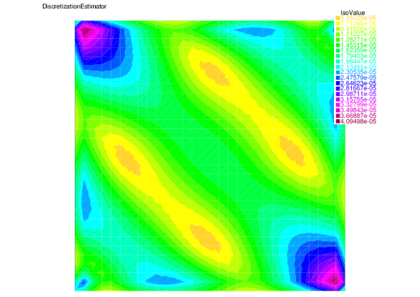
4) with this equilibrated flux, we can compute our estimator
Ph0 fh1,fh2;
fh1=f1;
fh2=f2;
// computation for the estimator
varf indicatorEtaDisc(unused,chiK) = int2d(Th)(chiK*(Div(u1,u2)'*Div(u1,u2))/beta/beta)
+  int2d(Th)(chiK*hTriangle*hTriangle/pi/pi*((f1-fh1)*(f1-fh1)+(f2-fh2)*(f2-fh2)))
+  int2d(Th)(chiK*(  ([dx(u1),dy(u1),dx(u2),dy(u2)]-[d11,d12,d21,d22]-[p,0,0,p])'*([dx(u1),dy(u1),dx(u2),dy(u2)]-[d11,d12,d21,d22]-[p,0,0,p])));
Whh mapEtaDisc;
mapEtaDisc[]=indicatorEtaDisc(0,Whh);
real GlobalEstimator=sqrt(mapEtaDisc[].sum);
mapEtaDisc=sqrt(mapEtaDisc);
plot(mapEtaDisc,  ps="MapDiscretisationEstimator.eps",value=1, fill=1,cmm="DiscretizationEstimator");
In order to showcase the performance of the estimator, we consider an example with an analytic solution,
real beta = 0.44;    // to be change with each different case
func ue1=2*x^2*y*(x - 1)^2*(y - 1)^2 + x^2*y^2*(2*y - 2)*(x - 1)^2;
func ue2=- 2*x*y^2*(x - 1)^2*(y - 1)^2 - x^2*y^2*(2*x - 2)*(y - 1)^2;
func pe=x+y-1;
func dxue1=2*x*y^2*(2*y - 2)*(x - 1)^2 + 2*x^2*y*(2*x - 2)*(y - 1)^2 + x^2*y^2*(2*x - 2)*(2*y - 2) + 4*x*y*(x - 1)^2*(y - 1)^2;
func dyue1=2*x^2*y^2*(x - 1)^2 + 2*x^2*(x - 1)^2*(y - 1)^2 + 4*x^2*y*(2*y - 2)*(x - 1)^2;
func dxue2=- 2*x^2*y^2*(y - 1)^2 - 2*y^2*(x - 1)^2*(y - 1)^2 - 4*x*y^2*(2*x - 2)*(y - 1)^2;
func dyue2=- 2*x*y^2*(2*y - 2)*(x - 1)^2 - 2*x^2*y*(2*x - 2)*(y - 1)^2 - x^2*y^2*(2*x - 2)*(2*y - 2) - 4*x*y*(x - 1)^2*(y - 1)^2;
func f1=-24*x^4*y + 12*x^4 + 48*x^3*y - 24*x^3 - 48*x^2*y^3 + 72*x^2*y^2 - 48*x^2*y + 12*x^2 + 48*x*y^3 - 72*x*y^2 + 24*x*y - 8*y^3 + 12*y^2 - 4*y + 1;
func f2=48*x^3*y^2 - 48*x^3*y + 8*x^3 - 72*x^2*y^2 + 72*x^2*y - 12*x^2 + 24*x*y^4 - 48*x*y^3 + 48*x*y^2 - 24*x*y + 4*x - 12*y^4 + 24*y^3 - 12*y^2 + 1;
// Exact error computation
fespace Whh(Th,P0);
varf indicatorErrorDiscu(unused,chiK) = int2d(Th)(chiK*((Grad(uh1)-[dxue1,dyue1])'*(Grad(uh1)-[dxue1,dyue1])+(Grad(uh2)-[dxue2,dyue2])'*(Grad(uh2)-[dxue2,dyue2]) ));
varf indicatorErrorDiscp(unused,chiK) = int2d(Th)(chiK*(beta*beta* (ph-pe)'*(ph-pe)   ));
Whh mapErrorDisc;
Whh mapErrorDiscu, mapErrorDiscp;
mapErrorDiscu[]=indicatorErrorDiscu(0,Whh);
mapErrorDiscp[]=indicatorErrorDiscp(0,Whh);
real GlobalErrorU=sqrt(mapErrorDiscu[].sum);
real GlobalErrorP=sqrt(mapErrorDiscp[].sum);
mapErrorDiscu=sqrt(mapErrorDiscu);
mapErrorDiscp=sqrt(mapErrorDiscp);
mapErrorDisc=mapErrorDiscu+mapErrorDiscp;
-
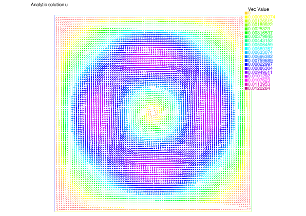
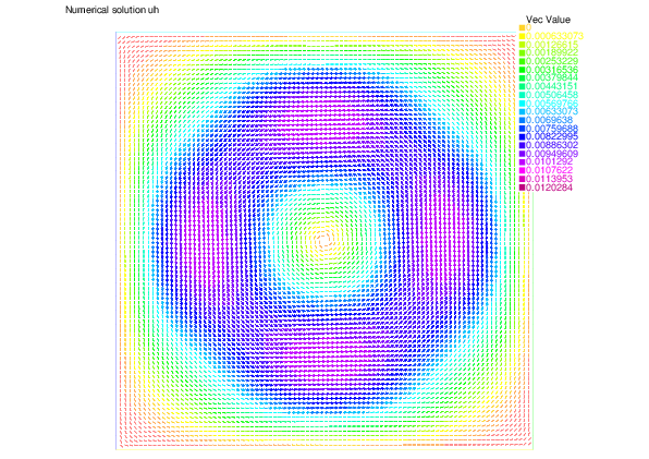
We show here the analytic velocity $\mathbf{u}$, the numerical velocity $\mathbf{u}_h$ by the finite element method, and the discretization error in velocity $\|\mathbf{u}-\mathbf{u}_h\|$
 |
 |
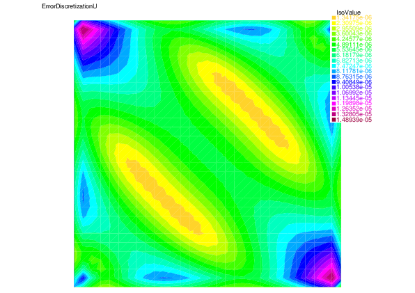 | |
| Analytic velocity $\mathbf{u}$ | Numerical velocity $\mathbf{u}_h$ | Discretization error in velocity $\|\mathbf{u}-\mathbf{u}_h\|$ |
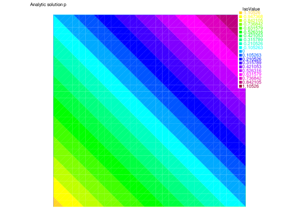
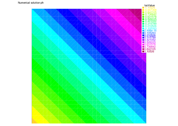
We show here the analytic pressure $p$, the numerical pressure $p_h$ by the finite element method, and the discretization error in pressure $\beta\|p-p_h\|$.
 |
 |
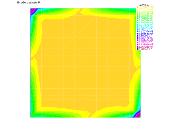 | |
| Analytic pressure $p$ | Numerical pressure $p_h$ | Discretization error in pressure $\beta\|p-p_h\|$. |
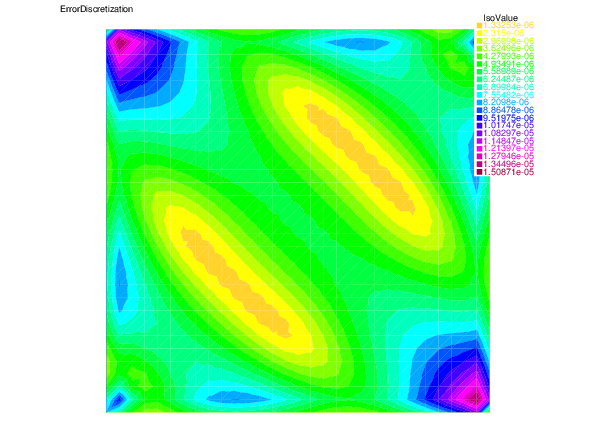
And in the end, we show the distribution of the total discretization error and the estimator, as well as the used mesh.
 |
 |
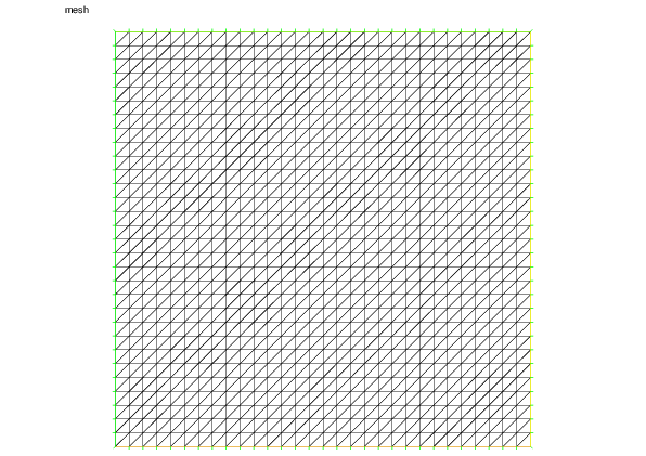 | |
| total Discretization error $\|\mathbf{u}-\mathbf{u}_h\|+\beta\|p-p_h\|$ | Discretization estimator | mesh |
With five levels of uniform mesh refinement, the effectivity index (the ratio between the total estimator and the total error) is given as follows:
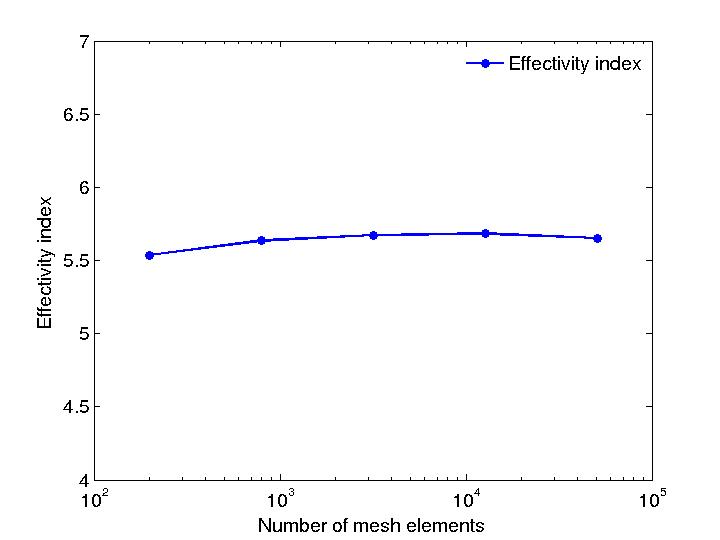 | |
| Effectivity index |
download the script: StokesEstimator.edp or return to main page