
Projects
preAlps
As part of NLAFET project, I have implemented a parallel E (nlarged) C (onjugate) G (radient) in C and MPI inside the preAlps library which is developped in Alpines team.
Features:
- Matrix and preconditioner free (Reverse Communication Interface)
- Very light: it only needs BLAS and LAPACK (Intel MKL)
- Documentation and examples
- Parallel performances assessed on different types of matrices
Download and install:
- Unfortunately the code is not available yet... but it should be released very soon!
Basic example:
 1 // Allocate memory and initialize variables
 2 preAlps_ECGInitialize(&ecg,rhs,&rci_request);
 3 // Finish initialization:
 4 // 1) P <- A*R
 5 preAlps_BlockJacobiApply(ecg.R,ecg.P);
 6 // 2) AP <- A*P
 7 preAlps_BlockOperator(ecg.P,ecg.AP);
 8 // Main loop
 9 while (stop != 1) {
10   preAlps_ECGIterate(&ecg,&rci_request);
11   // AP <- A*P
12   if (rci_request == 0) preAlps_BlockOperator(ecg.P,ecg.AP);
13   else if (rci_request == 1) {
14     // Check convergence
15     preAlps_ECGStoppingCriterion(&ecg,&stop);
16     if (stop == 1) break;
17     // Z <- M^-1 * R
18     if (ecg.ortho_alg == ORTHOMIN) preAlps_BlockJacobiApply(ecg.R,ecg.Z);
19     // Z <- M^-1 * AP
20     else if (ecg.ortho_alg == ORTHODIR) preAlps_BlockJacobiApply(ecg.AP,ecg.Z);
21   }
22 }
23 // Retrieve solution and free memory
24 preAlps_ECGFinalize(&ecg,sol);
Past Projects
Bocop
Bocop is an optimal control toolbox.
Features
- Windows/Mac/Linux compatible
- User friendly GUI
- Open Source
Work done: an HJB approach
This new algorithm is based on the resolution of the Hamilton-Jacobi-Bellman (HJB) equation associated to the optimal control problem. Indeed this equation characterizes the solutions of the optimal control problem.
Toy test: a mouse tries to get out the maze.
Academic projects
M.Sc.
Source code and documentation of those projects.
- 2D Helmholtz and wave equations solver
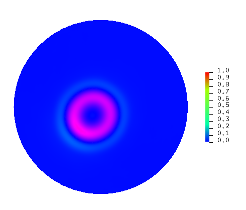
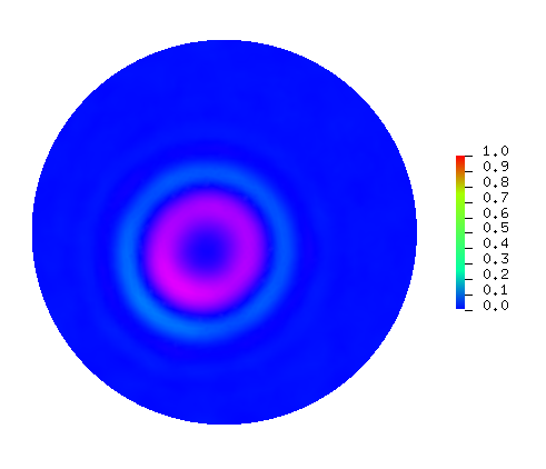
One example of a simulation obtained when solving the wave equation.
- 2D Navier-Stokes equations solver


Two examples of simulation: top, the viscosity of the fluid is 0.01 ; bottom, the viscosity of the fluid is 0.0025.
- Parallel low-rank decomposition
B.Sc.
- Building and programing a ball collector robot